3D instance segmentation with 3D-BoNet

Instance segmentation on point clouds is a challenging problem. Point clouds are unordered, sparse, non-uniform, and finding non-regulars shapes is not trivial. Moreover, the number of points in a scene can easily surpass the million, making every algorithm on point clouds very computationally expensive. The 3D-BoNet architecture [1] has been introduced recently to tackle the problem. This network is trainable end-to-end, and it mixes the results of a bounding box prediction branch with the output of a semantic segmentation branch to perform instance segmentation. The article contains a walkthrough of the paper, section by section, and eventually introduces our implementation in TensorFlow 2 obtained refactoring the original code in TensorFlow 1.

If you're not interested in the walkthrough of the paper, you can directly jump at the implementation.

Introduction

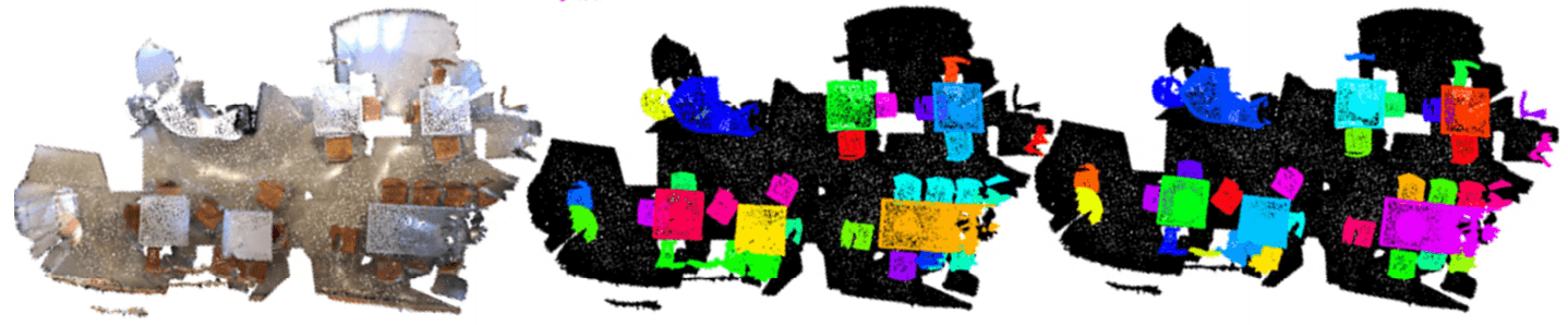
Instance segmentation is the natural intersection between object detection and semantic segmentation. Object detection tries to identify instances within the point cloud, while semantic segmentation assigns a semantic class to every point in the cloud. Instance segmentation aims to classify every point like semantic segmentation, but now distinct objects from the same semantic class have different labels. For this reason, an instance segmentation model should be able to reason over multiple scales: it has to recognize fine details to classify the points correctly, and, at the same time, it has to take into account objects in their entirety.

Analysis of point clouds is burdensome because point clouds are inherently unordered, unstructured, and non-uniform. The approaches to work with point clouds can be divided into three families: projection-based, discretization-based, and point-based methods. In projection-based methods, the point cloud is projected to a plane, and the resulting image is analyzed with image processing techniques. Discretization-based approaches organize points in a grid of voxels summarizing the point features in voxels. This discretization allows using 3D convolutional neural networks because it imposes a regular geometric structure. The main drawback of this representation is its memory footprint, which can be very high if the scene covers a large section of space.

The 3D-BoNet approach is point-based like SGPN [2], ASIS [3], JSIS3D [4], MASC [5], 3D-BEVIS [6], but all these methods do not explicitly detect object boundaries (i.e, the bounding boxes). Furthermore, they require computationally intensive post-processing, such as mean-shift clustering.

Unlike previous models, 3D-BoNet directly regresses the vertices of instance bounding boxes. Then, it selects the points belonging to the instance applying a binary classifier to the points within the bounding box. For doing this, the authors introduced a bounding box prediction module and a series of carefully designed loss functions to directly learn object boolean masks.

The pure 3D-BoNet method does not require post-processing, but it only works on small point clouds, usually composed of 4096 points. It is necessary to split the cloud into spatial blocks to manage more numerous point clouds. A spatial block contains the points belonging to a rectangular parallelepiped with square base. The number of points in a block is constant to allow the creation of batches. For this reason, from a single spatial block, many processing blocks are created by sampling points.

Architecture

The architecture is very similar to a traditional architecture used on images: backbone (feature extractor) and different heads for multi-task learning.

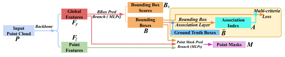
The input point cloud $\textbf{P} \in \mathbb{R}^{N \times k_0}$ has $N$ points and $k_0$ feature channels (such as the location coordinates $\{x,y,z\}$ and color $\{r,g,b\}$). The backbone network extracts point local features $\textbf{F}_l \in \mathbb{R}^{N \times k}$, where $k$ is the length of feature vectors. Then, local features are aggregated in a global feature vector $\textbf{F}_g \in \mathbb{R}^{1 \times k}$.

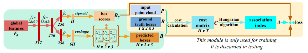
The Bounding Box Prediction Branch (BBPB) takes global features $\textbf{F}_g$ as input and regresses a predefined and fixed set of bounding boxes $B$ and the corresponding box scores $B_s$.

During the training, this branch is supervised with ground truth boxes. The bounding box association layer associates the most similar predicted bounding box to every ground truth box. The output of the association layer is a list of indices $\textbf{A}$ that describes the best pairing between boxes. Paired boxes are then compared with a multi-criteria loss. The bounding box association layer and multi-criteria loss (the content of the yellow box in the figure) are discarded for inference.

In parallel with the BBPB, predicted boxes, local features $\textbf{F}_l$ and global features $\textbf{F}_g$ are fed into the Point Mask Prediction Branch (PMPB).

Bounding Box Prediction Branch (BBPB)

The goal of the BBPB is to predict a bounding box for each instance in a single forward pass without relying on predefined spatial anchors or RPN (Region Proposal Network). A bounding box is parametrized by a pair of opposed vertices: $\{ [x_\text{min}, y_\text{min}, z_\text{min}], [x_\text{max}, y_\text{max}, z_\text{max}]\}$

As for all detection tasks, the number of total instances is variable. The BBPB gets around this problem by predicting a fixed number of bounding boxes together with confidence scores. At inference time, only the boxes with a high confidence score are retained.

Since the instances have no natural order, they are predicted in random order. For this reason, it is not trivial how to link predicted bounding boxes with ground truth labels to supervise the network. Given a set of ground truth instances, we need to determine which predicted boxes best fit them. This problem can be formulated as an optimal assignment and solved using an existing solver.

To supervise the network during the training, the authors introduce a bounding box association layer that relies on the Hungarian algorithm to perform the association. A multi-criteria loss pushes the network to minimize the distance between paired boxes. At the same time, the loss promotes the maximization of the coverage of instance points inside predicted boxes.

Bounding Box Association Layer

Given $H$ predicted bounding boxes $\textbf{B} \in \mathbb{R}^{H \times 2 \times 3}$ how can we use ground truth bounding boxes $\bar{\textbf{B}} \in \mathbb{R}^{T \times 2 \times 3}$ to supervise the network?

The Bounding Box Association Layer associates to every $T$ ground truth box one of the $H$ predicted boxes when $T \leq H$. When $T > H$, the largest $H$ ground truth boxes only are retained.

The associations between boxes can be encoded in a boolean association matrix $A \in \mathbb{R}^{H \times T}$ such that $\textbf{A}_{i,j} = 1$ if and only if the $i^{\text{th}}$ predicted bbox is assigned to the $j^{\text{th}}$ ground truth box. At the same time the dissimilarity between any pair of boxes can be stored in the cost matrix $\textbf{C} \in \mathbb{R}^{H \times T}$. Hence, the box association problem is to find the optimal assignment matrix $\textbf{A}$ with the minimal cost overall: $\mathbf{A} = \text{argmin}_{A} \sum_{i=1}^{H}{\sum_{j=1}^{T}{C_{i,j}A_{i,j}}}$ subject to $\sum_{i=1}^{H}{A_{i,j}} = 1, \sum_{j=1}^{T}{A_{i,j}} \le 1, j \in {1,\ldots,T}, i \in {1,\ldots, H}$ The problem above is an instance of the linear assignment problem, thus it can be solved with the Hungarian algorithm.

To evaluate the dissimilarity between the $i^\text{th}$ predicted bounding box and the $j^\text{th}$ ground truth box, the Euclidean distance between corresponding vertices is not enough because nearby bounding boxes cover a very different amount of points associated with an instance. Thus, the coverage of instance points should be included in the cost matrix $\textbf{C}$ to distinguish between similar boxes. The final association cost is the sum of 3 values.

1. Euclidean Distance between bounding boxes. A bounding box $B_i$ is represented by the coordinates of a pair of opposed vertices, so $B_i \in \mathbb{R}^6$ and we can define a distance between bounding boxes using the Euclidean distance in $\mathbb{R}^6$:

   $C^{ed}_{i,j} = \frac{1}{6}\sum{(B_i - \overline{B}_j)^2}.$

2. Soft IoU on Points. For every point of the point cloud, we can establish if it falls inside a bounding box or not. Thus, for a ground truth bounding box, we can compute a hard-binary vector $\overline{q}\in \{0, 1\}^N$ that for every point associates the value 1 if the point is inside the box or the value 0 if it is outside.

   The cost has to be a differentiable function of the predicted bounding boxes. For this reason, we define a differentiable version of $\overline{q}$ (named $q$) for predicted boxes. The vector $q \in [0, 1]^N$ is called point-in-pred-box-probability and its $n^\text{th}$ element is a function of the distance of the $n^\text{th}$ point from the vertices of the bounding box such that the deeper the point is inside of the box, the higher the value.

3. Cross-Entropy Score. The cross-entropy score between $q_i$ and $\overline{q}_j$ counterbalances the sIoU: the sIoU cost favors tighter boxes, while the cross-entropy prefers larger and more inclusive boxes.
   It is formally defined as:

   $C^\text{ces}_{i,j} = - \frac{1}{N}\sum_{n=1}^N{[\bar{q}_j^n \log q_i^n + (1 - \bar{q}_j^n)\log(1-q_i^n)]}$

The final association cost between the $i^\text{th}$ predicted bounding box and the $j^\text{th}$ ground truth box is defined as:

$C_{i,j} = C^{ed}_{i,j} + C^{\text{sIoU}}_{i,j} + C^{\text{ces}}_{i,j}.$

The entries in the cost matrix $\mathbf{C}$ are filled according to this formula and the association matrix $\mathbf{A}$ is computed through the Hungarian algorithm.

Loss Functions

The association matrix $\mathbf{A}$ allows reordering the predicted boxes, placing them in correspondence with the most similar ground truth box. The reordered bounding boxes can then be compared with ground truth bounding boxes using a differentiable loss function. The loss function that supervises the model is composed of two parts.

Multi-criteria Loss for Box prediction. We reuse and minimize the association cost previously defined, i.e.

$\mathcal{l_\text{bbox}} = \frac{1}{T} \sum_{t=1}^{T}{C^{ed}_{t,t} + C^{\text{sIoU}}_{t,t} + C^{\text{ces}}_{t,t}}.$

Here we only minimize the cost of $T$ paired boxes, while the remaining $H-T$ boxes are ignored. In practice, $\mathcal{l_\text{bbox}}$ corresponds to the minimal cost found by the Hungarian algorithm.

Loss for Box Score Prediction. The predicted box scores $B_s$ aim to indicate the validity of the corresponding predicted boxes. During training target score is 1 for the first reordered $T$ box and 0 for the remaining $H-T$. We can thus use the cross-entropy loss for this binary classification task:

$\mathcal{l_\text{bbs}} = -\frac{1}{H} \left[ \sum_{t=1}^{T}{B^t_s} + \sum_{t=T+1}^{H}{\log(1- B^t_s)} \right]$

This loss rewards correctly predicted bounding boxes and implicitly penalizes multiple similar boxes covering the same instance. During inference, box scores determine the number of instances detected in the point cloud: in fact, the accepted bounding boxes are the ones whose box score exceeds a given threshold.

Point Mask Prediction Branch

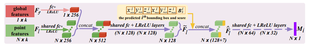
Given the predicted boxes $\mathbf{B}$, the point features $F_l$ and the global features $F_g$, the Point Mask Prediction Branch processes each bounding separately with shared neural layers to establish which points inside the bounding box belong to the detected instance.

For the $i^\text{th}$ predicted bounding box $B_i$ the estimated vertices and score are fused with processed features $\tilde{F}_l$ through concatenation, producing a box-aware features $\widehat{F}_l$. These features are then fed through shared layers terminating with a sigmoid activation function, predicting a point-level probability mask, denoted as $M_i$. The full branch architecture is detailed in the figure above.

The predicted instance masks $M$ are associated with the ground truth masks according to the association matrix $\mathbf{A}$. Due to the imbalance of instance and background points, the focal loss with default hyper-parameters is used instead of standard cross-entropy loss. As in the bounding box prediction branch, only the valid $T$ paired masks are used for the loss $\mathcal{l_\text{pmask}}$.

Semantic Segmentation and Instance Segmentation

The 3D-BoNet architecture can be adapted to perform semantic segmentation along with object detection. The semantic segmentation task is a pointwise prediction task like the point mask prediction task. Thus, the semantic segmentation branch is very similar to the point mask prediction branch. The difference is that the output is a multi-class probability vector instead of a binary probability value. This branch of the network is trained using a pointwise softmax cross-entropy loss function $\mathcal{l_\text{sem}}$.

The combination of the two tasks gives the instance segmentation of the scene. The bounding box prediction branch identifies the instances in the point cloud, while the semantic segmentation branch classifies every point in a single semantic class. The instance segmentation of the scene is obtained by assigning to every instance the most common semantic label predicted for its points.

In conclusion, the final instance segmentation model is trained end-to-end using a single combined multi-task loss:

$\mathcal{l_\text{all}} = \mathcal{l_\text{sem}} + \mathcal{l_\text{bbox}} + \mathcal{l_\text{bbs}} + \mathcal{l_\text{pmask}}.$

Management of Large Point Clouds

The 3D-BoNet framework is based on pointwise predictions. This property can be problematic when the point cloud to be analyzed is composed of millions of points, because the memory consumption of a single forward pass can easily exceed the memory available on a GPU. The problem is even more relevant during training when gradients have to be stored along with layer outputs. For this reason, it is necessary to devise a strategy to train and use the model on large point clouds.

Subsampling

First of all, it is always a good idea to subsample the point cloud to remove points in highly dense regions. There are many methods to prune points in dense regions: in our implementation, the subsampling preserves only one point per voxel in a grid. More in detail, the 3D space of points is divided virtually into voxels by a cubic grid whose size is a parameter of the experiment. For every voxel, a single point is preserved. Its coordinates are obtained by averaging the coordinates of all points in the voxel.

This method is easy to implement, and it can reduce the number of points in the point cloud by one order of magnitude, but it is still not sufficient.

Block Merging

The authors of 3D-BoNet propose to use Block Merging [2] to split the point cloud into fixed-sized blocks of points. Let us see how blocks are created. First of all, the 3D space is partitioned in overlapping square-based parallelepipeds of infinite height. For example, for a dataset composed of rooms, the squared base of every column usually measures $1 \text{m}^2$, and the overlap between consecutive columns is usually $0.5 \text{m}$ in both directions. Afterward, several blocks are extracted from every column by sampling a fixed number of points, usually 4096.

The quality of the final prediction is heavily affected by Block Merging: the arbitrary division of the space can distribute the same instance over several columns, while the random subsampling can destroy local and global structures putting nearby points in different blocks. In particular, for large objects, the model is forced to focus on local structures only.

The splitting part of the Block Merging method is quite simple, but it is necessary to implement also the inverse procedure, the merging part of the algorithm. Given all the instances detected in every block, the merge procedure groups them if they overlap more than a certain threshold. To understand the details of the merging algorithm, let us suppose, for example, that a sofa spans two partially overlapping consecutive blocks. The first block covers the mid-left part of the sofa, and the right block includes the points on the mid-right side of the object. As for subsampling, the merging relies on a discretization of the 3D space in fixed-size voxels. A voxel can be empty or associated with a semantic class and an instance identifier. In the example, the 3D-BoNet model takes as input the first block and finds a single instance of the class sofa. Then, all voxels containing a sufficiently high number of points whose predicted label is "sofa" are marked as "sofa" voxel. Likewise, the identifier of a new global instance of the class "sofa" is attached to all such voxels. Such voxel assignments are never changed by following blocks: they will be part of the final prediction on the point cloud. The procedure above is repeated when the second block is analyzed. Since the second block overlaps with the first block in its left part, now some voxels have a class label and an instance identifier from the previous block. The merge of instances happens when many voxels shared by the two blocks are labeled with the same semantic label. If that occurs, the instance detected in the second block does not become a new instance, but it shares the identifier of the existing "sofa" instance. In this way, even if the object was divided into several blocks, it is possible to recompose it.

The procedure is visibly complex, and its output depends on the order of blocks. Moreover, since blocks are groups of arbitrary points, the output is not a deterministic function of the input point cloud and the model. Finally, the procedure is highly dependent on the size of the voxel, losing all the advantages provided by working directly on sparse points.

Implementation

The 3D-BoNet framework can be used in combination with any backbone: in our experiments, we implemented and used PointNet or PointNet++. Our implementation is directly inspired by the official implementation, but it has many advantages over the original code.

Our implementation:

• is compatible with TensorFlow 2, while the original code support TensorFlow 1 only;
• is organized into commented functions and classes;
• reduces the number of custom operations on point cloud from 3 to just 1, replacing custom operations that have to be compiled manually with native TensorFlow functions;
• implements the Block Merging method in TensorFlow, allowing to export it with the model in the SavedModel format simplifying the deployment of the model
• manages S3DIS and ScanNet datasets directly, and it allows the definition of custom datasets.

Our implementation obtains results comparable with the published ones for the S3DIS dataset. The S3DIS dataset is the only dataset compatible with the original code released, and, in addition, the authors of the 3D-BoNet paper have published the dataset in its processed form with the point clouds already split into blocks. The reproduction of the results on S3DIS is thus not very hard, but it also hides most of the challenges posed by Block Merging.

We have encountered much more problems while working with the ScanNet dataset. This dataset is composed of point clouds larger than the ones in S3DIS, requiring a heavy subsampling. Furthermore, the division into blocks has to be performed from scratch. The authors declare great detection results on ScanNet without releasing the necessary code to reproduce them, but we have not attained the stated results. Even after numerous experiments that cover a wide range of hyper-parameters for subsampling and Block Merging, our trained models obtain very low accuracy. This fact raises some doubt about the effectiveness of the 3D-BoNet framework for the segmentation of large point clouds.

You can find our implementation on Github: https://github.com/zurutech/3DBoNet2.

---

[1] Learning Object Bounding Boxes for 3D Instance Segmentation on Point Clouds

[2] SGPN: Similarity Group Proposal Network for 3D Point Cloud Instance Segmentation

[3] Associatively Segmenting Instances and Semantics in Point Clouds

[4] JSIS3D: Joint Semantic-Instance Segmentation of 3D Point Clouds with Multi-Task Pointwise Networks and Multi-Value Conditional Random Fields

[5] MASC: Multi-scale Affinity with Sparse Convolution for 3D Instance Segmentation

[6] 3D-BEVIS: Birds-Eye-View Instance Segmentation